Q-Learning House Navigation
Reinforcement learning is a relatively new field in machine learning,
with ties in control systems, decision theory, probability, and
simulation. A Markov Decision Process (MDP) is a process
that relies on previous information to make new decisions with maximum
probability of a meritorious outcome. One of the simplest algorithms to
compute this is called Value Iteration. We will be working
through this with a simple housing example where we hope to
learn the optimal policy that will navigate an agent
through the house. In general, these policies are often lodged in our
own mental models, but once put on paper (or in a matrix), they are a
lot more interesting, and sometimes calibrate even our own thinking.
After all, the field of Deep Reinfrocement Learning has
beaten renouned championed in chess, alpha-go, and even star craft. So
whatever it is learning in those deep models can certainly augment our
intelligence.
The simplicity of MCPs make them very interpretable, but at the cost of more power. So let’s take a look and see if we can cook up a function to solve the problem.
Value Iteration
The idea of value iteration is that it is a recursive function with a few well known things.
- S = State-space
- A = Action-space
- R = Reward function
The problem is set up as an objective. The real goal is to acquire a
policy that acts optimally. By acting optimally, this is
scoped to maximizing a univariate reward function. How is this done?
Let’s take a look at the math.
Value Iteration \[ Q(s_1,a_1)=R(s_1,a_1) + \gamma\sum_{s_2 \neq s_1 \in S}{P(s_2 | s_1, a_1) \: max(Q(s_2, a_2) \: \forall a_2 \in A)} \]
At each iteration, a reward is known, and the future reward is also calculated for every other state.
Bellman Equation \[ Q_{now}(s_1,a_1) = Q_{old}(s_1,a_1) +\alpha \: (r + \gamma \: max_{a_2}(s_2, a_2)-Q_{old}(s_1, a_1)) \]
The Bellman Equation is also well known for solving
problems like this, and it doesn’t require the transition probability
above.
The Problem
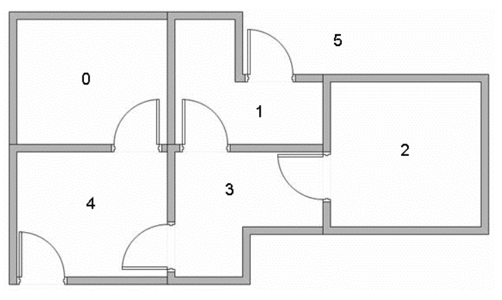
We hope to mimic a house navigation agent. The goal is to be able to review the optimal policy at the end that teaches the agent to travel from any room to any other room.
Reward Matrix
There are three criteria,
- -1 if “you can’t get there from here”
- 0 if the destination is not the target state
- 100 if the destination is the target state
R <- matrix(c(-1, -1, -1, -1, 0, 1,
       -1, -1, -1, 0, -1, 0,
       -1, -1, -1, 0, -1, -1,
       -1, 0, 0, -1, 0, -1,
        0, -1, -1, 0, -1, 0,
       -1, 100, -1, -1, 100, 100), nrow=6, ncol=6, byrow=TRUE) %>% t

R
[,1] [,2] [,3] [,4] [,5] [,6]
[1,] -1 -1 -1 -1 0 -1
[2,] -1 -1 -1 0 -1 100
[3,] -1 -1 -1 0 -1 -1
[4,] -1 0 0 -1 0 -1
[5,] 0 -1 -1 0 -1 100
[6,] 1 0 -1 -1 0 100tmp <- R %>% as.data.frame()
tmp <- tmp %>% dplyr::mutate(from = names(tmp))
tmp <- tmp %>% tidyr::gather(., key = "to", "reward", -from)
tmp <- tmp %>% dplyr::arrange(desc(reward))
ggplot(data = tmp) +
geom_tile(aes(x=from, y=to, fill=as.factor(reward))) +
labs(fill = "Reward") + theme_classic() +
ggtitle("Reward Matrix")
source("https://raw.githubusercontent.com/NicoleRadziwill/R-Functions/master/qlearn.R")

results <- q.learn(R,10000,alpha=0.1,gamma=0.8,tgt.state=6)
round(results)
[,1] [,2] [,3] [,4] [,5] [,6]
[1,] 0 0 0 0 80 0
[2,] 0 0 0 64 0 100
[3,] 0 0 0 64 0 0
[4,] 0 80 51 0 80 0
[5,] 64 0 0 64 0 100
[6,] 64 80 0 0 80 100The table produced tells us the average value to obtain policies. A
policy is a path through the states. One can quickly observe going from
room 0 to room 5 which is the solution. You
can walk through these and choose the argmax which along
the columns that provides the decision for your next row of choice.
tmp <- results %>% as.data.frame()
tmp <- tmp %>% dplyr::mutate(from = names(tmp))
tmp <- tmp %>% tidyr::gather(., key = "to", "reward", -from)
tmp <- tmp %>% dplyr::arrange(desc(reward))

ggplot(data = tmp) +
  geom_tile(aes(x=to, y=from, fill=reward)) +
  labs(fill = "Average Value (%)") + theme_classic() +
  ggtitle("Policy Decision Matrix") +
  scale_fill_gradient(low = "red", high = "green") +
  ylab("State From") +
  xlab("Action To")
Pretty cool!
Episilon-greedy
One common way of sampling an action is the
epislon-greedy approach. This tells us to exploit with
epsilon probability and randomly explore with 1-epsilon. Let’s take a
look.
q.learn.epsilon.greedy <- function(R, epochs = 10000, alpha = 0.1,gamma = 0.8, epsilon = 0.75,tgt.state = 6, testme = T){

  Q = matrix(0, nrow = nrow(R), ncol=ncol(R))

  epsilon.greedy <- function(state, Q, epsilon = 0.75, test = F){
    random_number <- runif(n = 1, min = 0, max = 1)
    if(random_number < epsilon){

      if(test)
        paste("exploit")
      else
        which.max(Q[state,])
    }
    else{

      if(test)
        paste("explore")
      else
        sample(which(Q[state, ] != state), 1)

    }
  }

  test.epsilon.greedy <- function(epsilon = 0.75){
    memory <- c()
    tmp <- c()
    for(j in 1:100){
      for(i in 1:100){
      # Start at a random state
      cs = sample(1:nrow(Q), 1)
      ns = epsilon.greedy(cs, Q, epsilon = epsilon, test = T)
      tmp <- c(tmp, ns) # we expect 75/100 to be exploits
      }
      memory <- c(memory, mean(tmp == "exploit"))
    }

    # looks good.
    memory %>% mean
  }

  # Test it
  if(testme){

    t1<-test.epsilon.greedy(epsilon=0.75)
    t2<-test.epsilon.greedy(epsilon=0.5)
    t3<-test.epsilon.greedy(epsilon=0.25)
    print(paste(round(t1,2)," == 0.75"))
    print(paste(round(t2,2)," == 0.50"))
    print(paste(round(t3,2)," == 0.25"))
  }


  learning_rate = alpha
  discount_rate = gamma
  dest.state = tgt.state

  for(i in 1:epochs){

    # Start at a random state
    cs = sample(1:nrow(Q), 1)
    cs

    while(TRUE){


        # Take an action
        a = epsilon.greedy(cs, Q, epsilon = 0.8, test = F)


        # Assess the reward
        r = R[cs, a]

        # Update policy matrix
        Q[cs, a] = learning_rate * (Q[cs, a]) + (1 - learning_rate) * (r + discount_rate * max(Q[a, ]) )
         # Q[cs,a] <- Q[cs,a] + learning_rate*(R[cs,a] + discount_rate*max(Q[a, ]) - Q[cs,a])

         # Update the current state
        cs = a


        if(a == dest.state){
          break
        }
    }
  }
  Q*100/max(Q)
}

Q = q.learn.epsilon.greedy(R, epochs = 10000, alpha = 0.1,gamma = 0.8, epsilon = 0.75, tgt.state = 6, testme=T)
[1] "0.75 == 0.75"
[1] "0.51 == 0.50"
[1] "0.26 == 0.25"idx = apply(Q, 1, which.max)
I <- matrix(0, nrow=nrow(Q), ncol=ncol(Q))
for(i in 1:nrow(I)){
I[i,idx[i]] = 1
}
I [,1] [,2] [,3] [,4] [,5] [,6]
[1,] 0 0 0 0 1 0
[2,] 0 0 0 0 0 1
[3,] 0 1 0 0 0 0
[4,] 0 1 0 0 0 0
[5,] 0 0 0 0 0 1
[6,] 0 0 0 0 0 1Our resulting matrix from an epsilon greedy algorithm
does something similar to the 100% exploit algorithm sourced in from the
github above. The policy is as follows:
- If in room 0 go to room 4, then to room 5 for the victory. (2 steps)
- If in room 4 go to room 5 for the victory. (1 step)
- If in room 1 go to room 5 for the victory. (1 step)
- If in room 2 go to room 1, then go to room 5 for the victory. (2 steps)
- If in room 3 go to room 1, then go to room 5 for the victory. (2 steps)
- If in room 4, go to room 5 for the victory. (1 step)
- If in room 5 .. victory! (0 steps)
For convenience, an indicator matrix is also built to illustrate the best possibile choice to and from any state with zero ambiguity. At a glance, outside of room 5, room 1 is a favorable place to be. It seems like it discovered a good outlet to arrive at the optimal, that is not optimal itself. Very interesting!
References